Definition of an electricity supply system
General tool structure
The electricity supply system can be defined de-/activating a number of available system components in the input template excel file. The technical specifications used can be defined in this input file and can also undergo a sensitivity analysis. The input data to be provided includes:
Demand profiles for multiple project sites
Weather data (irradiation, wind speed, temperature) of a project site
Technical specifications of fossil-fuelled generator, PV, wind and storage unit
Costs for the fossil-fuelled generator, PV, wind and storage unit
The input data is then pre-processed, e.g. the specific CAPEX and OPEX of each asset is calculated. If necessary, a randomized blackout profile is generated. From this, the tool defines the electricity system model using oemof and optimizes it for each of the sensitivity experiments. The results are evaluated, calculating main performance indicators (supply reliability, Levelized Costs of Electricity (LCOE), renewable share)) and generating automated graphs of the electricity flows within the system.
The simulation tool outline is provided with the graph below:
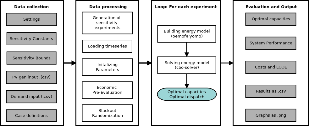
Flowchart of the micro grid simulation tool Offgridders
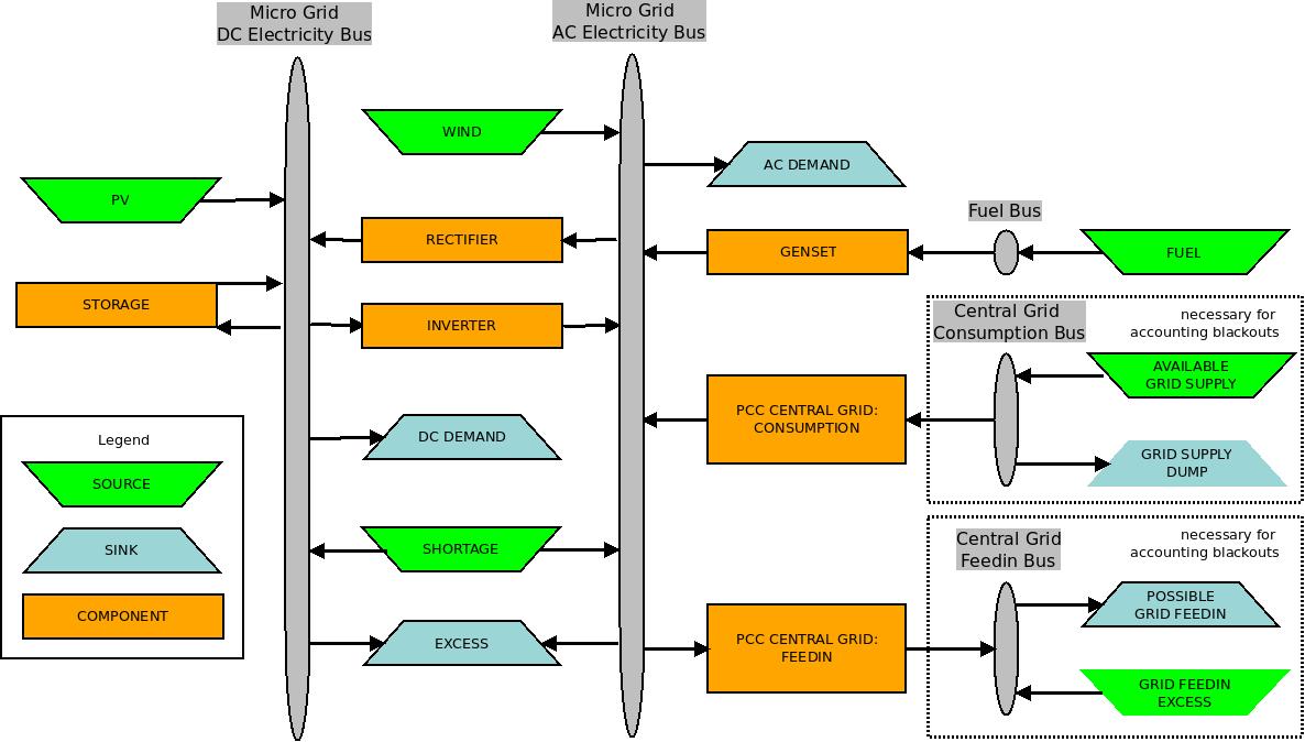
Electricity supply system components
To model and optimize energy systems, and specifically MG’s, an AC- as well as DC-bus with a multitude of components are integrated in the tool. A visualization of the tool’s structure can be found below. The components and their technological parameters shall be presented in the proceeding paragraphs.
Connected to the DC-bus are the following components:
PV plant, modelled based on a feed-in time series in kWh/kWp installed. The installed capacity in kWp can be optimized. Efficiency and system losses are not parameters of the simulation, but rather have to be included in the provided time series.
Battery storage, modeled with a constant throughput-efficiency, maximum charge- and discharge per time step defined through attributed C-rates, as well as minimal and maximal SOC. The installed capacity (kWh) and power output (kW) can be optimized.
DC demand as a time series in kWh.
Excess and shortage sink required due to oemof-terminology.
Through a rectifier and inverter with defined conversion efficiency, the DC- bus is connected to an AC-bus with following components:
Wind plant, modelled based on a feed-in time series in kWh/kW installed. The installed capacity kW can be optimized.
Generator, modelled with a constant efficiency and with or without minimal loading. The generator type is determined by the combustion value of the used fuel. The installed capacity in kW can be optimized. The capacity of a generator with minimal loading can not be optimized. Fuel usage is detected trough a fuel source.
Point of Common Coupling, enabling consumption from and/or feed-in to central grid. The installed capacity in kW can be optimized. Costs can either be attributed to the grid operator or the utility grid operator. The Point of Common Coupling (PCC) can allow an electricity flow only when the grid is available. This is defined through a Boolean time series, in which 1 indicates grid availability and 0 an outage.
AC demand as a time series in kWh.
Excess and shortage sink required due to oemof-terminology.
It is possible to optimize the dispatch of fixed capacities or to determine the optimal capacities of an energy system with or without connection to a central grid. It is not possible to directly define the used component capacities, apart from the diesel generator and the PCC, both of which can be sized based on a ratio of peak demand.
In the Electricity supply system, almost all assets can be de-activated. The assest can be seeing in following figure: